Backpropagation Part 1 : The What

Introduction

In Part 5, we traced the journey of data through a neural network. We saw how forward propagation takes input features and transforms them into predictions. But we left a crucial question unanswered.

"Network ne prediction toh kar di par ye khud ko improve kaise karega??"

Forward propagation tells us what the network thinks. But to make the network learn, we need to tell it how wrong it is and use that information to improve. This is where Backpropagation comes in.

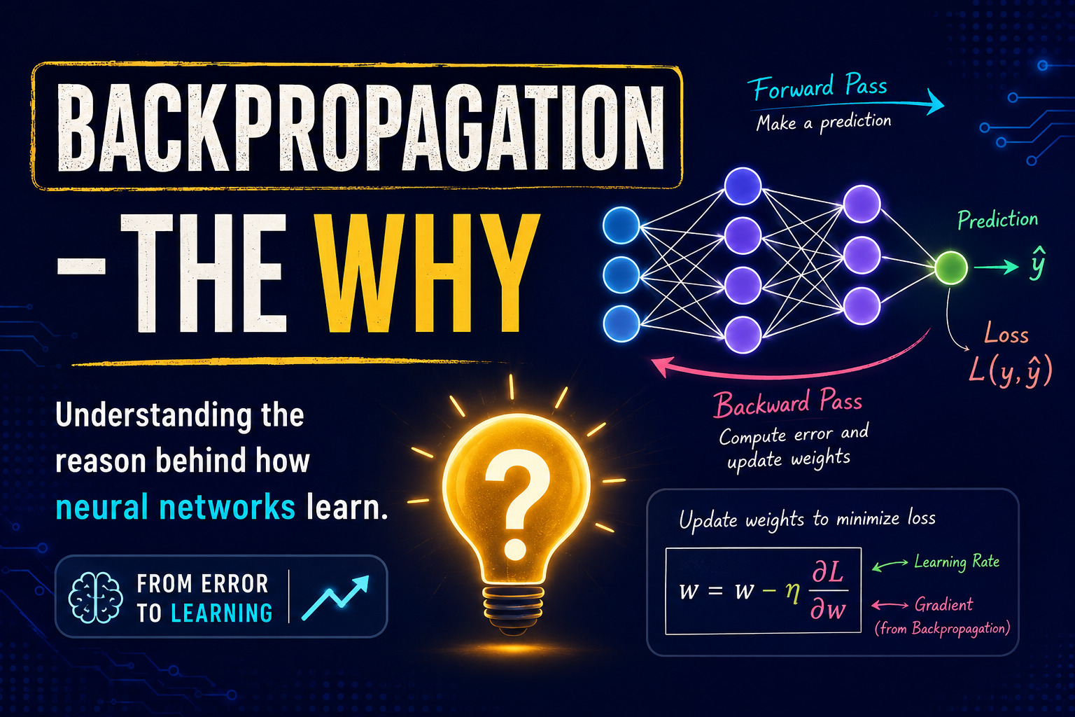
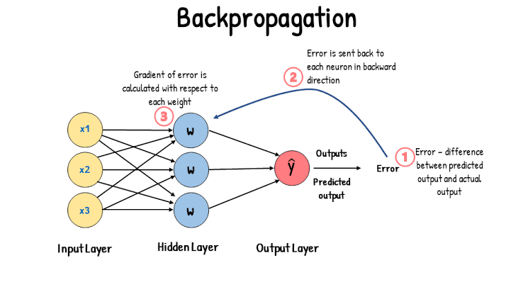
Backpropagation, short for "Backward Propagation of Errors," is the learning algorithm that trains Artificial Neural Networks. It works by propagating the error from the output layer backward toward the input layer and updating the weights and biases using Gradient Descent.

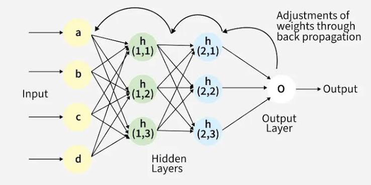
In simple words:

Forward Propagation → Calculate Loss → Backward Propagation → Update Weights and Biases

"Yahi hai Backpropagation. Isi wajah se neural networks data se seekh paate hain."

Before we dive deep, let's understand the prerequisites you need to grasp this concept fully.

Prerequisites

Before understanding Backpropagation, you should be familiar with:

1. Forward Propagation

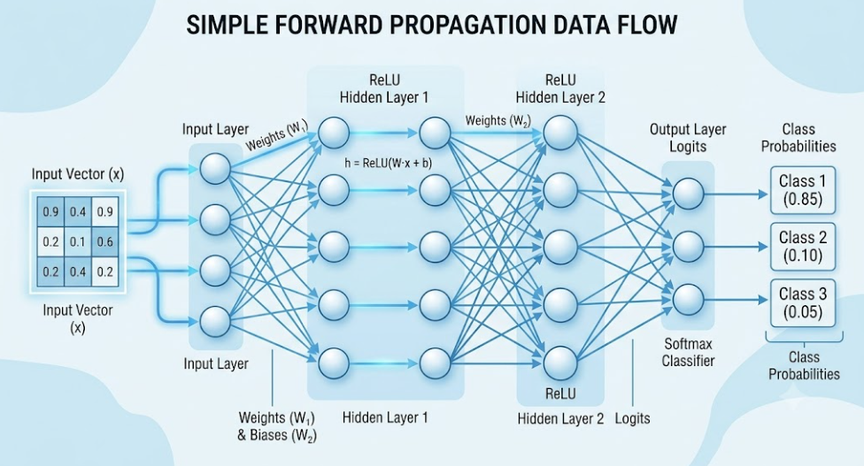
Forward propagation is the process of passing input data through a neural network to generate an output. We covered this in detail in Part 5.

In forward propagation:

• Data enters the input layer

• Passes through hidden layers

• Produces a prediction at the output layer

• Each neuron computes: z = Σ(w_i × x_i) + b and applies an activation function

If you haven't read Part 5 yet, I highly recommend going through it first. Forward propagation is the first half of Backpropagation.

"Forward propagation samjhe bina, Backpropagation nahi samajh aayega."

2. Gradient Descent

Gradient Descent is the optimization algorithm that minimizes the loss function by adjusting weights and biases.

The core idea is simple:

Weight_new = Weight_old - η × ∂Loss/∂Weight

Bias_new = Bias_old - η × ∂Loss/∂Bias

Where:

• η (eta) is the learning rate — a small number that controls how big the steps are

• ∂Loss/∂Weight is the gradient — it tells us how much the loss changes when we change the weight

"Gradient Descent batata hai ki kis direction mein move karna hai to reduce the loss."

Think of it like finding the lowest point in a valley. The gradient tells you which direction is downhill, and the learning rate tells you how big a step to take.

3. Partial Derivatives

A partial derivative measures how a function changes when we change one variable while keeping others constant.

For a loss function L(w₁, w₂), the partial derivative ∂L/∂w₁ tells us:

• How much does L change when w₁ changes slightly?

• Keeping w₂ fixed

"Partial derivative batata hai ki ek specific parameter change karne se loss kitna change hota hai."

4. Chain Rule of Differentiation

The chain rule is the mathematical foundation of Backpropagation. It allows us to compute the gradient of the loss with respect to weights in earlier layers.

If y depends on u, and u depends on x, then:

dy/dx = (dy/du) × (du/dx)

In neural networks:

Loss depends on Prediction → Prediction depends on Hidden Output → Hidden Output depends on Weight

So to find how the loss changes with a weight in an early layer, we multiply the gradients along the path.

"Chain rule hi Backpropagation ka heart hai."

Working of Backpropagation

Let's understand Backpropagation step by step using a simple regression example.

The Dataset

Suppose we have the following regression dataset:

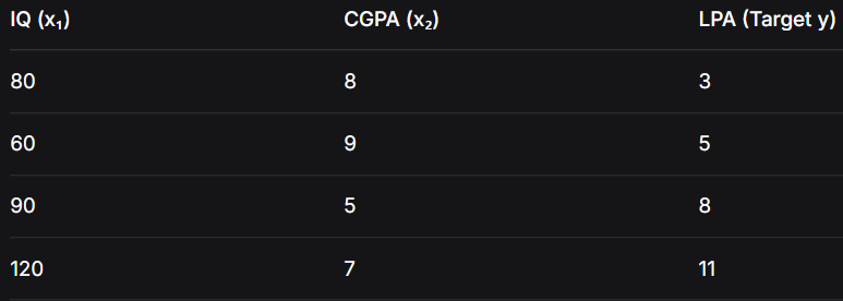
Here:

• Input features: x₁ = IQ, x₂ = CGPA

• Output: y = LPA (package in Lakhs Per Annum)

Step 1: Select One Training Example

Backpropagation processes one training example at a time (or a mini-batch).

Let's take the first example:

• IQ = 80, CGPA = 8

• Target y = 3

"Ek example lete hain, aur uske liye pura process samajhte hain."

Step 2: Initialize Weights and Biases

Initially, all weights and biases are randomly initialized.

For this example, let's use simple values:

• All weights = 1

• All biases = 0

But remember, in real scenarios, weights are initialized with small random numbers.

Step 3: Perform Forward Propagation

Now we pass the input through the neural network.

Network Architecture:

• Input Layer: 2 neurons (IQ, CGPA)

• Hidden Layer: 2 neurons (h₁, h₂)

• Output Layer: 1 neuron

Hierarchy of Dependency of Features, Weights and Biases on the Output:

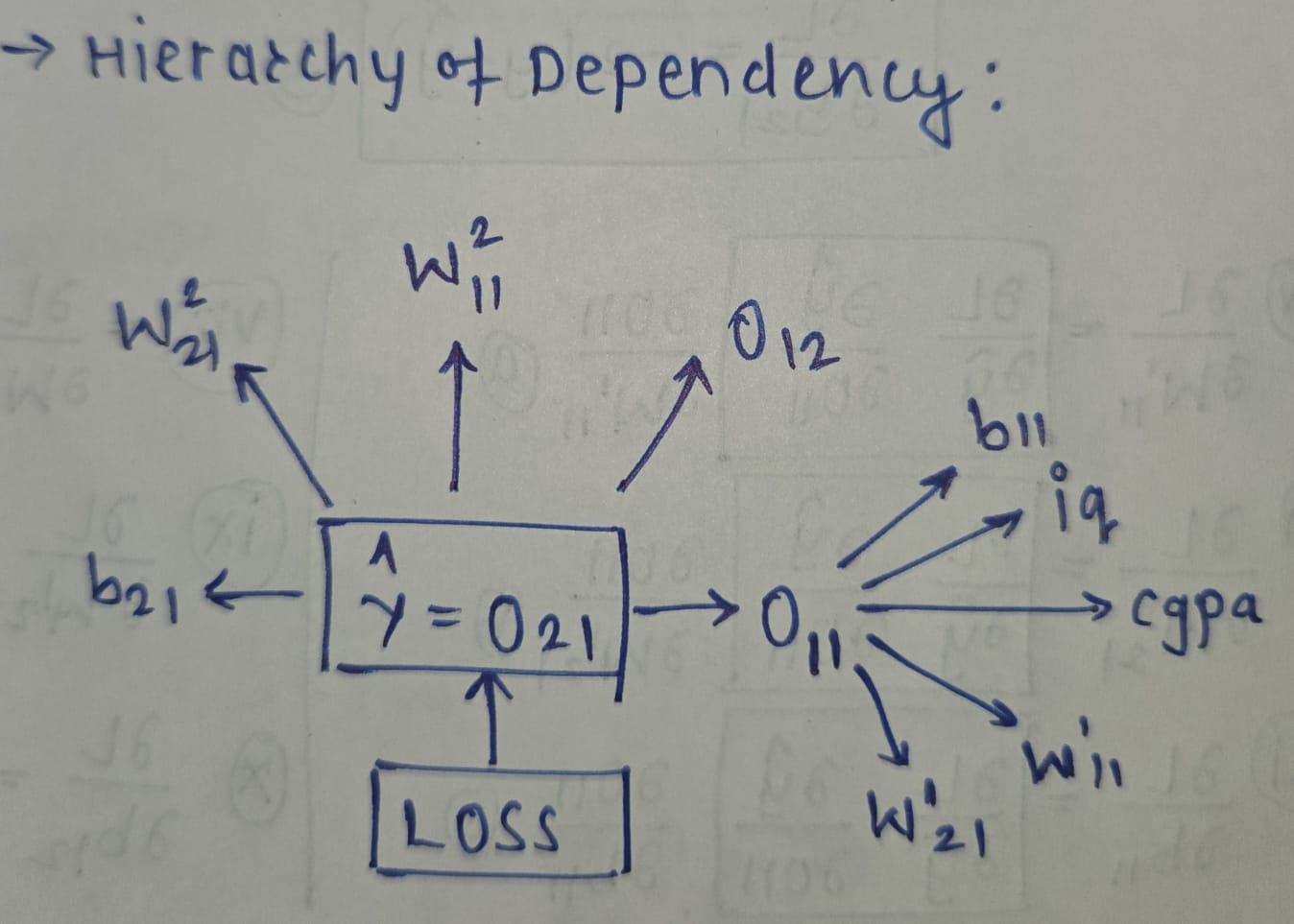
Hidden Layer Computation:

For hidden neuron h₁:

o₁₁ = x₁ × w₁₁(¹) + x₂ × w₂₁(¹) + b₁₁

o₁₁ = 80 × 1 + 8 × 1 + 0

o₁₁ = 88

For hidden neuron h₂:

o₁₂ = x₁ × w₁₂(¹) + x₂ × w₂₂(¹) + b₁₂

o₁₂ = 80 × 1 + 8 × 1 + 0

o₁₂ = 88

Since this is a regression problem, we use a linear activation function (no activation).

Output Layer Computation:

ŷ = o₁₁ × w₁₁(²) + o₁₂ × w₂₁(²) + b₂₁

ŷ = 88 × 1 + 88 × 1 + 0

ŷ = 176

"Forward propagation ne prediction diya: 176, but actual value hai 3. Bahut bada error hai!"

Step 4: Calculate Loss

Since this is a regression problem, we use Mean Squared Error (MSE).

For one sample:

L = (y - ŷ)²

L = (3 - 176)²

L = (-173)²

L = 29929

The loss is huge! Now we need to update weights to reduce this loss.

"Itna bada loss, ab weights update karke isko kam karna hai."

Step 5: Update Weights and Biases

This is where Backpropagation shines. We use Gradient Descent to update every trainable parameter.

Weight update:

W_new = W_old - η × ∂L/∂W_old

Bias update:

b_new = b_old - η × ∂L/∂b_old

The key challenge is computing ∂L/∂W for every weight in the network.

Why Do We Need Derivatives?

The derivative tells us how much the loss changes when a parameter changes.

For any weight:

∂L/∂W

Means: "How much does the loss change if this particular weight changes?"

"Yeh gradient batata hai ki weight ko kis direction mein move karna hai."

If ∂L/∂W is positive:

• Increasing W increases L

• So we should decrease W

If ∂L/∂W is negative:

• Increasing W decreases L

• So we should increase W

Dependency Between Loss and Weights

Consider weight w₁₁(²) (the weight connecting hidden neuron h₁ to the output).

Notice that w₁₁(²) does not directly affect the loss.

Instead:

w₁₁(²) → ŷ → L

• Changing the weight changes the prediction

• Changing the prediction changes the loss

Therefore, using the Chain Rule:

∂L/∂w₁₁(²) = ∂L/∂ŷ × ∂ŷ/∂w₁₁(²)

"Yahi Chain Rule hai. Isse hum earlier layers ke gradients compute kar paate hain."

Breaking Down the Chain Rule

1. Derivative of Loss

Loss function:

L = (y - ŷ)²

Differentiate with respect to prediction:

∂L/∂ŷ = -2(y - ŷ)

For our example:

∂L/∂ŷ = -2(3 - 176) = -2(-173) = 346

2. Gradient of Output Layer Weights

Prediction equation:

ŷ = o₁₁ × w₁₁(²) + o₁₂ × w₂₁(²) + b₂₁

For weight w₁₁(²):

∂ŷ/∂w₁₁(²) = o₁₁ = 88

Therefore:

∂L/∂w₁₁(²) = ∂L/∂ŷ × ∂ŷ/∂w₁₁(²)

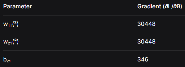
∂L/∂w₁₁(²) = 346 × 88 = 30448

For weight w₂₁(²):

∂ŷ/∂w₂₁(²) = o₁₂ = 88

Therefore:

∂L/∂w₂₁(²) = 346 × 88 = 30448

For output bias b₂₁:

∂ŷ/∂b₂₁ = 1

Therefore:

∂L/∂b₂₁ = 346 × 1 = 346

Backpropagating to Hidden Layer

Now we move one layer backward. This is where Backpropagation gets its name.

For hidden neuron h₁:

o₁₁ = x₁ × w₁₁(¹) + x₂ × w₂₁(¹) + b₁₁

Loss depends on w₁₁(¹) through:

w₁₁(¹) → o₁₁ → ŷ → L

Using the Chain Rule:

∂L/∂w₁₁(¹) = ∂L/∂ŷ × ∂ŷ/∂o₁₁ × ∂o₁₁/∂w₁₁(¹)

We already know:

∂L/∂ŷ = 346

Now:

∂ŷ/∂o₁₁ = w₁₁(²) = 1

And:

∂o₁₁/∂w₁₁(¹) = x₁ = 80

Therefore:

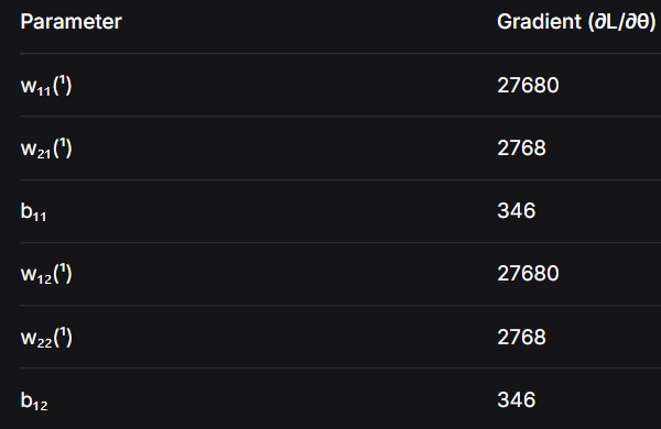
∂L/∂w₁₁(¹) = 346 × 1 × 80 = 27680

"Gradient hidden layer tak pahunch gaya!"

All Hidden Layer Gradients

For weight w₂₁(¹):

∂o₁₁/∂w₂₁(¹) = x₂ = 8

∂L/∂w₂₁(¹) = 346 × 1 × 8 = 2768

For hidden bias b₁₁:

∂o₁₁/∂b₁₁ = 1

∂L/∂b₁₁ = 346 × 1 × 1 = 346

For weight w₁₂(¹):

∂ŷ/∂o₁₂ = w₂₁(²) = 1

∂o₁₂/∂w₁₂(¹) = x₁ = 80

∂L/∂w₁₂(¹) = 346 × 1 × 80 = 27680

For weight w₂₂(¹):

∂o₁₂/∂w₂₂(¹) = x₂ = 8

∂L/∂w₂₂(¹) = 346 × 1 × 8 = 2768

For hidden bias b₁₂:

∂o₁₂/∂b₁₂ = 1

∂L/∂b₁₂ = 346 × 1 × 1 = 346

Summary of All Gradients

Output Layer

Hidden Layer

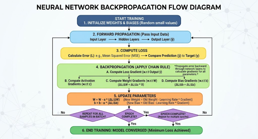
Complete Backpropagation Algorithm

Now let's put it all together in a step-by-step algorithm:

1. Initialize all weights and biases randomly.

2. Select one training example (or a mini-batch).

3. Perform Forward Propagation to obtain the prediction ŷ.

4. Compute the Loss using an appropriate loss function (MSE for regression, Cross-Entropy for classification).

5. Calculate Gradients for every trainable parameter using the Chain Rule:

   • Start from the output layer

   • Propagate gradients backward through the network

   • Use the Chain Rule to compute gradients for earlier layers

6. Update each weight and bias using Gradient Descent:

   θ_new = θ_old - η × ∂L/∂θ

7. Repeat steps 2-6 for all training samples.

8. One complete pass over the entire dataset is called an epoch.

9. Continue training for multiple epochs until the loss converges (reaches a minimum).

"Yeh process repeat hota hai jab tak loss minimum na ho jaaye."

What We Learned

In this "What" part of Backpropagation:

1. Backpropagation is the algorithm that trains neural networks by propagating error backward.

2. The Chain Rule is the mathematical foundation that allows us to compute gradients for all parameters.

3. Gradients tell us how much the loss changes when we change each parameter.

4. Gradient Descent uses these gradients to update weights and biases.

5. Forward Propagation must be understood before Backpropagation makes sense.

6. Every parameter in the network gets updated during Backpropagation.

Things to keep in mind so that we can move forward to next part

1. Backpropagation = Forward Pass → Calculate Loss → Backward Pass → Update Weights

2. The Chain Rule is the mathematical backbone of Backpropagation.

3. Gradients are computed from the output layer backward to the input layer.

4. Every weight and bias in the network is updated using Gradient Descent.

5. Learning Rate controls how big the weight updates are.

6. The process repeats for multiple epochs until the loss converges.

Conclusion

Today we understood what Backpropagation is and how it works at a fundamental level. We traced the entire process: from forward propagation to loss calculation to gradient computation to weight updates.

"Yeh tha Backpropagation ka 'What' part."

We saw how the Chain Rule allows us to propagate error backward through the network. We computed gradients for every parameter in our example. We understood why each step is necessary for learning.

But we haven't answered two crucial questions:

• How does Backpropagation actually work in practice with activation functions like Sigmoid and ReLU?

• Why does Backpropagation work so well, and what are its limitations?

In the next part, we'll explore The How of Backpropagation. We'll implement it from scratch, see how activation functions affect gradients, and understand the mechanics of training in detail.

"Ab 'How' part mein hum Backpropagation ko implement karke dekhenge."

Then in Part 8, we'll dive into The Why and understand the mathematical intuition, the vanishing gradient problem, and why Backpropagation is the most important aspect of modern deep learning.

Stay tuned for Part 7: Backpropagation - The How!