Forward Propagation: How Information Travels Through a Neural Network

Introduction

In Part 4, we built Multi-Layer Perceptrons and saw how they can solve complex problems that single neurons cannot handle. We understood the architecture, the layers, and why depth matters. But we didn't look closely at what actually happens inside the network when we feed it data.

"Data andar jaata hai, prediction bahar aati hai, but beech mein kya hota hai?"

Today, we are going to trace the journey of a single data point as it travels through a neural network. Every number, every multiplication, every activation. This journey is called Forward Propagation, and it is the foundation of how neural networks make predictions.

Think of it like a package moving through a delivery network. The package enters at one point, passes through multiple sorting stations, gets processed at each station, and finally reaches its destination with a label attached. That label is the prediction.

What is Forward Propagation?

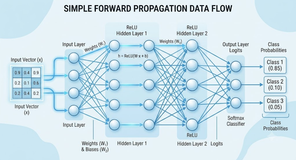
Forward propagation is the process of passing input data through a neural network to generate an output. It is called "forward" because information moves in only one direction. From the input layer, through the hidden layers, to the output layer.

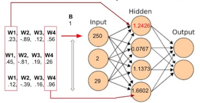
Every neuron in the network performs two simple operations:

Weighted Sum: Multiply each input by its weight, add them all up, and add the bias.
Activation: Pass the weighted sum through an activation function to produce the neuron's output.

This output then becomes the input for the next layer, and the process repeats until we reach the final output.

The Core Computation

For a single neuron with inputs x₁, x₂, ..., xₙ, weights w₁, w₂, ..., wₙ, and bias b:

Step 1: z = (w₁ × x₁) + (w₂ × x₂) + ... + (wₙ × xₙ) + b

Step 2: a = f(z)

Where f is the activation function (like ReLU, Sigmoid, or Tanh).

A Simple Analogy

Imagine you are a teacher grading students. You have three criteria:

Attendance (weight: 0.2)
Homework (weight: 0.3)
Exam Score (weight: 0.5)

A student comes with: Attendance = 90%, Homework = 80%, Exam = 85%

Your "weighted sum" would be:

z = (0.2 × 90) + (0.3 × 80) + (0.5 × 85)

z = 18 + 24 + 42.5

z = 84.5

Then you apply your "activation function" (your grading policy) to decide the final grade. If z >= 60, the student passes.

This is exactly what a neuron does. It takes inputs, multiplies them by weights, adds them up, and applies an activation function.

Step-by-Step Example

Let's trace a single data point through a small neural network. We'll use a 2-3-1 network:

2 input neurons (features)
1 hidden layer with 3 neurons
1 output neuron

The Data Point

We have a student with:

IQ = 110
CGPA = 8.5

Input vector: x = [110, 8.5]

The Weights and Biases

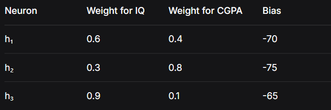
The network has learned these weights during training:

Hidden Layer (3 neurons)

Output Layer (1 neuron)

Forward Propagation: Step by Step

Step 1: Input Layer

The input layer simply passes the data forward without any computation.

x₁ = 110 (IQ)

x₂ = 8.5 (CGPA)

Step 2: Hidden Layer Computation

For hidden neuron h₁:

z₁ = (0.6 × 110) + (0.4 × 8.5) + (-70)

z₁ = 66 + 3.4 - 70

z₁ = -0.6

Apply ReLU activation: a₁ = max(0, -0.6) = 0

For hidden neuron h₂:

z₂ = (0.3 × 110) + (0.8 × 8.5) + (-75)

z₂ = 33 + 6.8 - 75

z₂ = -35.2

Apply ReLU activation: a₂ = max(0, -35.2) = 0

For hidden neuron h₃:

z₃ = (0.9 × 110) + (0.1 × 8.5) + (-65)

z₃ = 99 + 0.85 - 65

z₃ = 34.85

Apply ReLU activation: a₃ = max(0, 34.85) = 34.85

The hidden layer outputs are: a = [0, 0, 34.85]

Step 3: Output Layer Computation

For the output neuron:

z_output = (0.7 × 0) + (0.5 × 0) + (0.3 × 34.85) + (-0.5)

z_output = 0 + 0 + 10.455 - 0.5

z_output = 9.955

Apply Sigmoid activation:

y = sigmoid(9.955) = 1 / (1 + e⁻⁹·⁹⁵⁵) ≈ 0.9999

Since y > 0.5, we classify this as "Placed" (1).

Matrix Representation

In practice, neural networks use matrix multiplication for efficiency. The entire forward pass can be computed in one go.

Hidden Layer (Matrix Form)

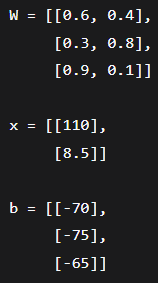
z = Wx + b

Where:

W is the weight matrix (3 × 2)
x is the input vector (2 × 1)
b is the bias vector (3 × 1)

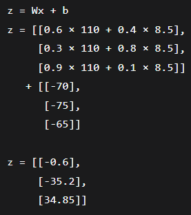
Apply ReLU: a = max(0, z) = [[0], [0], [34.85]]

Output Layer (Matrix Form)

z_output = W_output × a + b_output

Where W_output is (1 × 3) and a is (3 × 1)

z_output = [[0.7, 0.5, 0.3]] × [[0], [0], [34.85]] + [-0.5]

z_output = 9.955

Apply Sigmoid: y = sigmoid(9.955) = 0.9999

Forward Propagation in Action

Let's implement forward propagation on a real dataset. We'll use the Wisconsin Breast Cancer dataset.

The Code

[The Colab File with Code Implementation](https://colab.research.google.com/drive/1YWit53sm2YC9edFgSIDgMCtKnR5vPK8C?usp=sharing)

The Flow of Information

Let's summarize the forward propagation journey:

Step 1: Input Layer

Raw data enters the network
Each feature becomes an input neuron

Step 2: Hidden Layers

Each neuron computes: z = Σ(w_i × x_i) + b
Activation function is applied: a = f(z)
Output is passed to the next layer

Step 3: Output Layer

Same computation as hidden layers
Final activation depends on the problem:
- Binary classification: Sigmoid
- Multi-class classification: Softmax
- Regression: Linear (no activation)

The Result

A prediction (probability, class label, or continuous value)

Why Understanding Forward Propagation Matters

Understanding forward propagation is crucial because:

Debugging: When your model makes wrong predictions, tracing the forward pass helps identify where things go wrong.
Interpretability: Understanding what each layer does helps you interpret model decisions.
Architecture Design: Knowing how data flows helps you design better architectures.
Performance Optimization: Understanding the computation helps optimize for speed.
Foundation for Backpropagation: Forward propagation is the first half of training. Without understanding it, backpropagation (coming in Part 6) won't make sense.

Conclusion

Today we traced the journey of data through a neural network. We saw how each neuron multiplies inputs by weights, adds a bias, applies an activation function, and passes the result forward.

From the simple weighted sum to the final prediction, every step is a transformation. The input features become hidden representations, which become higher-level features, which finally become the prediction. This is how neural networks turn raw data into decisions.

In Part 6, we will reverse the flow. We will take the error and propagate it backward through the network.