Inside a Perceptron: A Step-by-Step Guide to How Machines Learn to Make Decisions

Introduction

In the first part of the series, we started an incredible journey. We explored the inspiration behind artificial intelligence, tracing its roots back to the human brain. We met the fundamental building block of neural networks, the Perceptron, and learned about Frank Rosenblatt's invention of Perceptron. We even built a simple, working perceptron in Python and got introduced to its famous limitation: the XOR problem.

It was like seeing a car for the first time and understanding what it does: it moves you from point A to point B. But today, we are going to open it's hood. We are going to open up the perceptron and look at every single component inside. We'll understand how it works, what each part does.

In this part of the series, we will dissect the perceptron piece by piece. We will explore how it takes in information, weighs its importance, makes a decision, and even learns from its mistakes. We will move from simple concepts to the mathematical framework that powers modern AI.

1. How Does a Perceptron Actually Work?

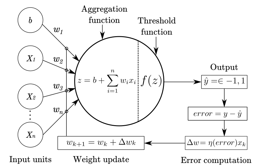
Before we get lost in the individual parts, let's get a bird's-eye view. A perceptron is a machine that makes binary decisions. Given a set of inputs, it produces a single output, usually a yes or no, a 1 or a 0. But how does it go from raw data to a final decision?

The process is a series of logical and mathematical steps, a pipeline through which data flows.

Socho ek factory ki assembly line. Raw materials (inputs) go in one end. As they move along the line, they are processed, evaluated, and combined. At the very end, a final product (the prediction) comes out. The "machinery" inside the perceptron that does this processing is the Weighted Sum and the Activation Function.

Rendering diagram...

At its core, the process is simple:

1. Input: The perceptron receives data, which we call features (x₁, x₂, ..., xₙ).
2. Weighted Sum: Each input is multiplied by a corresponding weight (w₁, w₂, ..., wₙ). These weights are the "knowledge" of the perceptron. A bias (b) is then added to this sum. This gives us a single number, z.
3. Activation: The number z is then passed through an Activation Function. This function acts like a gatekeeper, deciding the final output. For a classic perceptron, this gate is a Step Function. If z is greater than a certain threshold, the neuron "fires" (outputs 1), else it stays quiet (outputs 0).

2. Understanding Inputs: The Data That Fuels the Machine

The first step in the pipeline is getting the data. In the language of machine learning, data enters a model through Inputs.

A feature is an individual, measurable property of a phenomenon. In our case, features could be IQ and CGPA for a student placement prediction problem. An Input Vector is a collection of features for a single instance, often denoted as x.

For a student with an IQ of 110 and a CGPA of 8.5, the input vector would be [110, 8.5]. The number of features is called dimensionality. Our placement problem is 2-dimensional.

Real-World Data Examples

Let's look at how this concept applies in different domains.

Domain	Problem	Features (Input Vector)
Healthcare	Disease Diagnosis	Age, blood pressure, cholesterol, BMI, heart rate
Finance	Credit Scoring	Annual income, credit score, current debt, loan amount
Spam Detection	Email Classification	Presence of specific words, sender's domain, number of recipients

3. Understanding Weights: The Importance Multipliers

So, we have our raw data (inputs). A perceptron needs to learn which inputs are important and which aren't. It does this using Weights.

A weight is a simple number associated with a specific input. Think of it as the "importance multiplier" for that feature. The more important a feature is for the final decision, the larger its weight will be.

• High Positive Weight: As the value of this feature increases, the likelihood of the output being 1 also increases.
• High Negative Weight: As the value of the feature increases, the likelihood of the output being 1 decreases.
• Zero Weight: The feature has absolutely no influence on the decision.

4. Understanding Bias: The "Default" Decision

Now, let's consider a crucial question: What if all features are zero? Or what if we want to shift the decision boundary away from the origin? This is where the Bias (b) comes into play.

The bias is an additional constant parameter in the weighted sum. It's like a baseline, a "default decision" that we can shift to make the model more flexible.

Why Weights Alone Are Not Enough

Imagine a simple perceptron with one input. Its decision rule is: If (w₁ * x₁) > threshold, output 1, else 0. Let's say our threshold is 0. This rule will always output 0 when x₁ is 0. The decision boundary passes through the origin. What if our data is such that even when x₁ is 0, the correct output should be 1? We can't change the rule's offset without a bias.

Analogy for Bias

Think of a university exam. The weights are the importance of each subject. The bias is the passing percentage. Without a bias, a student who scores a perfect zero in all subjects would still pass. The passing percentage shifts the line that determines who passes.

Mathematically, the bias is just another weight that we add to the summation. It's often represented as w₀ multiplied by a constant input of 1.

5. Weighted Sum: The Calculation

Now, we put it all together. The Weighted Sum is the core computation of a perceptron. It combines the inputs and their weights, adds the bias, and produces a single number. This number, z, is then passed to the activation function.

The formula is:

z = w₁x₁ + w₂x₂ + ... + wₙxₙ + b

For our placement problem, this translates to:

z = (Weight_IQ * IQ) + (Weight_CGPA * CGPA) + Bias

Numerical Example

• Student Data: IQ = 110, CGPA = 8.5
• Weights: Weight_IQ = 0.6, Weight_CGPA = 0.4
• Bias: b = -70

z = (0.6 * 110) + (0.4 * 8.5) + (-70)
z = 66 + 3.4 - 70
z = -0.6

This student's weighted sum is -0.6. The activation function would then see that -0.6 < 0, so the output would be 0. The model predicts "Not Placed."

6. Activation Functions: Adding Life to the Model

So, we have z, a single number. For a binary classification, we want to map z to a 0 or 1. This is where the Activation Function comes in. The activation function takes z and squashes it into a specific range.

"Agar activation function na ho, toh pura network ek simple linear equation jaisa ho jayega. Usse complex problems nahi solve ki ja sakti."

An activation function introduces non-linearity. It allows the model to create complex decision boundaries and learn much more hidden relationships in the data.

a. The Step Function: The Classic Gatekeeper

The Step Function is the simplest activation function. It works as a strict, hard threshold.

f(z) = 1 if z >= 0
f(z) = 0 if z < 0

b. The Sigmoid Function: The Smooth Probabilistic Switch

The Sigmoid Function transforms z into a smooth S-shaped curve that ranges from 0 to 1.

f(z) = 1 / (1 + e⁻ᶻ)

Properties

• Output Range: (0, 1). It squashes the output to a probability between 0 and 1.
• Smooth and Differentiable: This is its biggest advantage over the step function.
• Derivative: f'(z) = f(z) * (1 - f(z)).

Advantages and Disadvantages

Advantages:

• Probabilistic interpretation.
• Smooth gradient for training.

Disadvantages:

• Vanishing Gradient: For very large positive or negative values of z, the gradient becomes extremely small.

c. The Tanh Function: The Zero-Centered Sibling

The Tanh function is similar to sigmoid, but its output range is from -1 to 1. It is zero-centered.

f(z) = tanh(z) = (eᶻ - e⁻ᶻ) / (eᶻ + e⁻ᶻ)

Advantages and Disadvantages

Advantages:

• Zero-centered, leading to more stable gradients.
• Stronger gradients compared to sigmoid.

Disadvantages:

• Still suffers from the vanishing gradient problem.

d. The ReLU Function: The Modern Game Changer

The Rectified Linear Unit (ReLU) is the most important activation function in modern deep learning.

f(z) = max(0, z)

Advantages and Disadvantages

Advantages:

• Computationally efficient.
• No vanishing gradient for positive values.

Disadvantages:

• Dying ReLU Problem: Neurons can become inactive and stop learning.

e. The Softmax Function: For Multi-Class Classification

The Softmax function is designed for multi-class classification. It takes a vector of raw values and transforms them into a probability distribution.

f(z)ᵢ = eᶻⁱ / Σⱼ eᶻʲ

Applications

Softmax is used in the output layer for any multi-class classification task, such as image classification or handwriting recognition.

7. Activation Function Comparison Table

Function	Formula	Output Range	Advantages	Disadvantages	Applications
Step	1 if z>=0 else 0	{0, 1}	Extremely simple	Non-differentiable, limited to linear problems	Basic logic gates
Sigmoid	1 / (1 + e⁻ᶻ)	(0, 1)	Probabilistic interpretation	Vanishing gradient	Binary classifiers
Tanh	(eᶻ - e⁻ᶻ)/(eᶻ + e⁻ᶻ)	(-1, 1)	Zero-centered	Vanishing gradient	Hidden layers
ReLU	max(0, z)	[0, ∞)	Efficient, no vanishing gradient	Dying ReLU problem	Deep networks, CNNs
Softmax	eᶻⁱ / Σ eᶻʲ	(0, 1)	Probability distribution	Sensitive to outliers	Multi-class classifiers

8. The complete Prediction Pipeline Architecture for student placement problem

Now, let's bring everything together. This is the complete journey of data through a perceptron.

Rendering diagram...

1. A Student's Data is collected, providing the Input Vector (x). For our placement case, x = [IQ, CGPA].
2. These inputs are multiplied by their respective Weights (w), learned from previous training data.
3. The Bias (b) is added to the product sum.
4. This results in a single value: the Weighted Sum (z).
5. The value z is passed through an Activation Function (f), which decides the final output.
6. The Prediction (e.g., Placed or Not Placed) is made.

This pipeline is the core of the perceptron's decision-making process.

9. Conclusion: A Glimpse into the Future

We've traveled a long way today. We opened the black box of the perceptron, looked at every component, and understood how it makes decisions. We explored various activation functions, each with its own strengths and weaknesses. We built a perceptron from scratch and understood its training process.

But here's the thing.

A single perceptron, no matter how well-tuned its weights and bias are, has a fatal flaw. It can only draw a straight line in the sand. It can solve simple problems like AND and OR, but it completely fails on one of the simplest logical problems ever created: the XOR problem.

If perceptrons are so powerful and form the basis of deep learning, why do they fail so spectacularly on XOR? How do we overcome this limitation?

"Isi point par humara asli deep learning journey shuru hota hai."

We need to build networks of perceptrons, stacked on top of each other, to learn complex, non-linear patterns. We need to move from a single layer to multiple layers. We need to create Multi-Layer Perceptrons (MLPs) . And to train them, we need a revolutionary algorithm called Backpropagation.

In the next part of this series, we will tackle the XOR problem head-on. We will build a multi-layer network that solves it, and we will unlock the true power of deep learning.

Get ready. The real adventure is just beginning. See you in Part 3!