Multi-Layer Perceptrons: Teaching Machines Complex Thinking

Introduction

In Part 3, we hit a wall. The XOR problem showed us that a single neuron, no matter how carefully we tune its weights and bias, simply cannot learn certain patterns. It was a humbling moment for early AI researchers.

"Agar ek neuron fail ho sakta hai, toh phir deep learning kaise possible hai?"

The answer lies in something beautifully simple yet profoundly powerful: stacking neurons together in layers. Just like a team of people can solve problems that no single person can tackle alone, a network of neurons working together can learn patterns that are impossible for a single perceptron.

This is where the journey from "perceptron" to "deep learning" truly begins. Welcome to the world of Multi-Layer Perceptrons (MLPs).

What is a Multi-Layer Perceptron?

A Multi-Layer Perceptron is exactly what it sounds like. A perceptron with multiple layers. But calling it just "multiple perceptrons" would be an understatement. An MLP is a feedforward neural network where neurons are arranged in layers, and information flows in only one direction. From input to output.

The Architecture

Think of an MLP like a multi-stage assembly line in a factory.

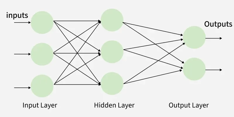
Input Layer is where raw data enters the network. Each neuron in this layer represents one feature of your data. For example, IQ, CGPA, or pixel values of an image.

Hidden Layers are the "thinking" layers of the network. They don't directly interact with the outside world. They are "hidden" between input and output. The magic happens here. Each hidden layer learns to recognize increasingly complex patterns in the data.

Output Layer produces the final prediction. Whether a student is placed, whether an image contains a cat, or which digit a handwritten character represents.

"Hidden layer hi asli deep learning ka raaz hai."

A defining characteristic of MLPs is that they are fully connected. Every neuron in one layer connects to every neuron in the next layer. This is why they are sometimes called "dense" neural networks.

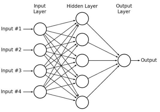
The diagram above shows a typical MLP structure with an input layer, one hidden layer, and an output layer. Each circle represents a neuron, and each line represents a connection with a weight.

Why Depth Matters: The Power of Hierarchy

You might be wondering: if a single neuron can't solve XOR, why does adding more layers help?

The Linear Limitation

Remember the step function from Part 2? A single perceptron calculates:

z = w₁x₁ + w₂x₂ + b

This is a linear equation. The decision boundary is a straight line. If your data can't be separated by a single straight line, like XOR, a single perceptron will always fail.

"One layer = one straight line. Two layers = many lines working together."

The Hidden Layer Solution

When we add a hidden layer, something extraordinary happens. The hidden layer transforms the original input space into a new representation where the problem becomes linearly separable.

For XOR, a two-layer network can decompose the problem:

XOR = (OR) AND (NOT AND)

h₁ = OR gate (detects if either input is 1)
h₂ = NAND gate (detects if not both inputs are 1)
Output = AND(h₁, h₂)

In this transformed space, the output layer can now draw a straight line to separate the classes.

Feature Discovery

Here is the truly remarkable thing. The hidden layer learns its own features. Nobody tells the network what features to look for. It discovers them automatically from the data.

First hidden layer: Detects simple patterns (edges, corners)
Second hidden layer: Combines simple patterns into complex features (shapes, objects)
Deeper layers: Recognizes high-level concepts (faces, scenes, categories)

This is called representation learning, and it is the secret behind deep learning's success. The network invents its own features instead of waiting for an expert to hand-design them.

The Universal Approximation Theorem

There is a beautiful mathematical result that explains why MLPs are so powerful. The Universal Approximation Theorem.

This theorem states that a feedforward neural network with a single hidden layer containing a finite number of neurons, and with a non-linear activation function, can approximate any continuous function to any desired degree of accuracy.

In plain English: if you have enough neurons in one hidden layer, you can learn almost any pattern.

"Ek hidden layer kaafi hai, but enough neurons hona chahiye."

Unfortunately, the theorem doesn't tell us how many neurons we need. A single hidden layer with a huge number of neurons might work, but in practice, using multiple hidden layers with fewer neurons is often more efficient and performs better.

Activation Functions in MLPs

We covered activation functions in detail in Part 2, but let's refresh why they are especially important in MLPs.

The Non-Linearity Requirement

Without non-linear activation functions between layers, a multi-layer network would behave exactly like a single-layer network. This is because multiple linear transformations can be combined into a single linear transformation.

"Activation function ke bina, layers useless hain."

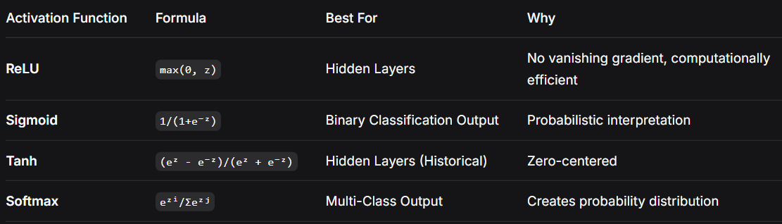
Modern MLPs typically use ReLU for hidden layers because it avoids the vanishing gradient problem and is computationally cheap. For the output layer, Sigmoid (binary) or Softmax (multi-class) is used.

Mathematical Notation of an MLP

Let's formalize what happens inside an MLP. This notation will be useful as we build more complex networks.

Forward Propagation

For a single layer l with n neurons, the forward pass computes:

z_1 = w₁₁x₁ + w₁₂x₂ + ... + w₁ₙxₙ + b₁

z_2 = w₂₁x₁ + w₂₂x₂ + ... + w₂ₙxₙ + b₂

z_m = wₘ₁x₁ + wₘ₂x₂ + ... + wₘₙxₙ + bₘ

In vector form, this becomes much cleaner:

z = Wx + b

Where:

W is the weight matrix (m × n)
x is the input vector (n × 1)
b is the bias vector (m × 1)
z is the pre-activation output (m × 1)

Then we apply the activation function element-wise:

a = f(z)

Where a is the output of the layer.

For the Entire Network

For a network with L layers:

Layer 1: z₁ = W₁x + b₁, a₁ = f₁(z₁)

Layer 2: z₂ = W₂a₁ + b₂, a₂ = f₂(z₂)

Layer L: zₗ = Wₗaₗ₋₁ + bₗ, aₗ = fₗ(zₗ) = ŷ

Where:

x is the input
ŷ is the final prediction
Wᵢ, bᵢ, fᵢ are the weights, biases, and activation functions of layer i

"Yahi hai MLP ka mathematical framework."

Training an MLP: The Learning Process

We've seen how an MLP makes predictions. But how does it learn?

The Challenge

A single perceptron learns by adjusting its weights based on the error at the output. But in an MLP, the hidden layers are, well, hidden. We can't directly see their errors.

The Solution

The network learns through a process called backpropagation, which we'll cover in detail in Part 6. For now, understand that:

The network makes a prediction (forward pass)
It calculates how wrong it was (loss)
It propagates this error backward through the network
It updates all weights to reduce future errors

This process repeats thousands of times until the network learns the underlying patterns in the data.

"Error ko backward propagate karke, hidden layers bhi apni mistakes se seekhte hain."

Gradient Descent

The weight updates are performed using Gradient Descent, an optimization algorithm that finds the minimum of the error function:

Δw = -η × ∂Error/∂w

Where η is the learning rate. A parameter that controls how big the weight updates are. If it's too small, learning is slow. If it's too large, the network might become unstable.

Epochs and Batches

Training involves multiple passes through the dataset:

Epoch: One complete pass through the entire training dataset
Batch: A subset of the training data used for one weight update
Iteration: One batch pass

Modern MLPs use mini-batch gradient descent, which balances the efficiency of batch learning with the stability of stochastic learning.

MLP in Action: Iris Dataset Example

Let's see a complete MLP implementation using scikit-learn on a real dataset. We'll use the famous Iris dataset, which contains measurements of three species of iris flowers.

The goal is to classify flowers into three species:

Iris Setosa (0)
Iris Versicolor (1)
Iris Virginica (2)

Architecture of the MLP

For this problem, we'll use:

Input Layer: 4 neurons (one for each feature)
Hidden Layer 1: 10 neurons with ReLU activation
Hidden Layer 2: 8 neurons with ReLU activation
Output Layer: 3 neurons with Softmax activation (for multi-class classification)

The hidden layers transform the original 4 features into a new space where the three species become linearly separable. The ReLU activation introduces non-linearity, allowing the network to learn complex patterns.

Complete Implementation

Here is the complete code to train and evaluate an MLP on the Iris dataset:

Step 0: Import Required Libraries

import numpy as np

from sklearn.datasets import load_iris

from sklearn.model_selection import train_test_split

from sklearn.preprocessing import StandardScaler

from sklearn.neural_network import MLPClassifier

from sklearn.metrics import accuracy_score, classification_report, confusion_matrix

import matplotlib.pyplot as plt

Step 1: Load the dataset

iris = load_iris()

X = iris.data # Features (sepal length, sepal width, petal length, petal width)

y = iris.target # Target (0=setosa, 1=versicolor, 2=virginica)

print(f"Dataset shape: {X.shape}")

print(f"Number of samples: {len(X)}")

print(f"Number of features: {X.shape[1]}")

print(f"Number of classes: {len(np.unique(y))}")

print(f"Class names: {iris.target_names}")

Step 2: Split the data into training and testing sets

X_train, X_test, y_train, y_test = train_test_split(

X, y, test\_size=0.2, random\_state=42, stratify=y

)

print(f"\nTraining samples: {len(X_train)}")

print(f"Testing samples: {len(X_test)}")

Step 3: Scale the features

scaler = StandardScaler()

X_train_scaled = scaler.fit_transform(X_train)

X_test_scaled = scaler.transform(X_test)

print(f"\nFeature scaling complete")

Step 4: Create and train the MLP

mlp = MLPClassifier(

hidden\_layer\_sizes=(10, 8),  # Two hidden layers with 10 and 8 neurons

activation='relu',  # ReLU activation for hidden layers

solver='adam',  # Adam optimizer for training

alpha=0.001,  # L2 regularization strength

batch\_size=20,  # Mini-batch size

learning\_rate\_init=0.001,  # Initial learning rate

max\_iter=1000,  # Maximum number of iterations

random\_state=42,  # For reproducibility

verbose=True  # Print training progress

)

Train the model

print("\nTraining MLP on Iris dataset...")

mlp.fit(X_train_scaled, y_train)

print("Training complete!")

Step 5: Make predictions

y_pred_train = mlp.predict(X_train_scaled)

y_pred_test = mlp.predict(X_test_scaled)

Step 6: Evaluate the model

train_accuracy = accuracy_score(y_train, y_pred_train)

test_accuracy = accuracy_score(y_test, y_pred_test)

print(f"\nTraining Accuracy: {train_accuracy:.4f}")

print(f"Testing Accuracy: {test_accuracy:.4f}")

print("\nClassification Report (Test Set):")

print(classification_report(y_test, y_pred_test, target_names=iris.target_names))

Step 7: Confusion Matrix

cm = confusion_matrix(y_test, y_pred_test)

print("\nConfusion Matrix:")

print(cm)

Step 8: Test a single prediction

test_sample = X_test[0].reshape(1, -1)

test_sample_scaled = scaler.transform(test_sample)

prediction = mlp.predict(test_sample_scaled)

prediction_proba = mlp.predict_proba(test_sample_scaled)

print(f"\nSingle Sample Prediction:")

print(f"Sample features: {X_test[0]}")

print(f"Actual class: {iris.target_names[y_test[0]]}")

print(f"Predicted class: {iris.target_names[prediction[0]]}")

print(f"Prediction probabilities: {prediction_proba[0]}")

Step 9: Plot training loss

plt.figure(figsize=(8, 6))

plt.plot(mlp.loss_curve_)

plt.title('MLP Training Loss')

plt.xlabel('Iterations')

plt.ylabel('Loss')

plt.grid(True)

plt.show()

Expected Output

When you run this code, you should see something like:

Dataset shape: (150, 4)

Number of samples: 150

Number of features: 4

Number of classes: 3

Class names: ['setosa' 'versicolor' 'virginica']

Training samples: 120

Testing samples: 30

Feature scaling complete

Training MLP on Iris dataset...

Iteration 1, loss = 1.0156

Iteration 100, loss = 0.2854

Iteration 200, loss = 0.1217

Iteration 300, loss = 0.0618

Training complete!

Training Accuracy: 0.9917

Testing Accuracy: 0.9667

Confusion Matrix:

[[10 0 0]

[ 0 9 1]

[ 0 0 10]]

Single Sample Prediction:

Sample features: [5.5 2.4 3.7 1. ]

Actual class: versicolor

Predicted class: versicolor

Prediction probabilities: [0.0012 0.9876 0.0112]

Explanation of the Pipeline

Let's understand what happened in this process:

Step 1: Data Loading

We loaded the Iris dataset with 150 samples, each having 4 features. The target has 3 possible classes. This is a small but classic dataset that is perfect for learning.

Step 2: Train-Test Split

We divided the data into training (80%) and testing (20%) sets. The training set is used to teach the model, and the testing set is used to evaluate how well it performs on unseen data. The stratify parameter ensures that the class distribution is preserved in both splits.

Step 3: Feature Scaling

We scaled the features using StandardScaler, which transforms the data to have mean 0 and standard deviation 1. This is crucial for neural networks because features on different scales can cause the learning process to be unstable. Without scaling, features with larger values would dominate the weight updates.

Step 4: Training

We created an MLP with two hidden layers. Hidden Layer 1 has 10 neurons with ReLU activation. Hidden Layer 2 has 8 neurons with ReLU activation. The Output Layer has 3 neurons with Softmax activation (automatically set for multi-class).

The adam solver is an advanced optimization algorithm that adapts the learning rate for each weight. It is one of the best choices for training neural networks.

Step 5: Prediction

The trained model predicts labels for both training and test data. The output is the class index (0, 1, or 2).

Step 6: Evaluation

We measured accuracy, which is the proportion of correct predictions. We also used a classification report that shows precision, recall, and F1-score for each class. These metrics give a more complete picture of performance, especially when classes are imbalanced.

Step 7: Confusion Matrix

This shows exactly which classes were misclassified. In our example, one versicolor was misclassified as virginica, but all setosa and virginica samples were correctly classified.

Step 8: Single Prediction

We demonstrated how to make a prediction for a single new sample. The model outputs probabilities for each class, and we can see which class has the highest probability.

Step 9: Loss Visualization

We plotted the training loss over iterations. The loss should decrease steadily, indicating that the network is learning. If the loss plateaus early, we might need to increase the network capacity or adjust hyperparameters.

Why This MLP Works

The MLP works on the Iris dataset because:

Non-Linearity: The ReLU activations in hidden layers allow the network to learn non-linear decision boundaries, which are needed to separate the three species.
Feature Transformation: The hidden layers transform the original 4 features into a new 3-dimensional space where the classes are linearly separable.
Softmax Output: The Softmax activation ensures the outputs can be interpreted as probabilities, making it suitable for multi-class classification.
Sufficient Capacity: With 10 and 8 neurons in the hidden layers, the network has enough capacity to learn the patterns in the data without overfitting.

"Yeh MLP Iris dataset ko classify karna automatically seekh gaya, bina kisi explicit rules ke."

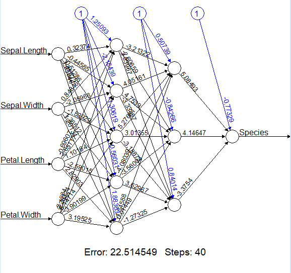
The flow above shows how the MLP trains. It starts with raw data, scales the features, initializes random weights, and then repeatedly performs forward passes, calculates loss, does backward passes, and updates weights until the loss reaches a minimum.

Why MLPs Succeed Where Single Perceptrons Fail

Let's summarize why MLPs are so much more powerful than single perceptrons:

Single Perceptron

Can only learn linear decision boundaries
Fails on non-linearly separable problems like XOR
Limited to simple problems
No feature learning capability

Multi-Layer Perceptron

Can learn complex, non-linear decision boundaries
Solves XOR and similar problems easily
Handles complex real-world problems
Learns its own features automatically

The key difference is the hierarchical feature learning. Each layer learns increasingly abstract features, combining simple patterns into complex concepts. This is why deep learning works.

"Yahi difference hai simple machine learning aur deep learning mein."

Choosing the Right Architecture

When building an MLP, several decisions need to be made:

Number of Hidden Layers

1 hidden layer: Can approximate any function (Universal Approximation Theorem)
2-3 hidden layers: Often works well for many problems
More layers: Needed for very complex problems like image recognition

Number of Neurons per Layer

Too few: Underfitting (can't learn patterns)
Too many: Overfitting (memorizes training data)
Rule of thumb: Start small and increase gradually

Activation Functions

Hidden layers: ReLU (default choice)
Output layer: Sigmoid (binary) or Softmax (multi-class)

Learning Rate

Too high: Network diverges
Too low: Slow convergence
Start with 0.001 and adjust based on loss curves

These choices are called hyperparameters. They are set before training and significantly affect the model's performance.

Conclusion

We have come a long way. From the single perceptron that struggled with XOR to a multi-layer network that can classify complex datasets like Iris. The addition of hidden layers wasn't just a small improvement. It was a paradigm shift that transformed artificial intelligence from a curiosity into a revolution.

The journey of MLPs has shown us how deep learning truly works. Layers of neurons, each learning its own features, working together to solve problems that are impossible for any single unit. The network learns to transform the data into a space where the problem becomes solvable. It discovers its own features. It creates its own understanding.

But our journey doesn't end here. We have built the architecture and understood its power. Now we need to understand how information flows through it. Every time we feed data into an MLP, a beautiful sequence of computations occurs. Each layer transforming the data, passing it forward, and gradually shaping it into the desired output.

In Part 5, we will zoom in on this process. We will follow a single piece of data as it travels through every neuron, every weight, every activation. We will understand Forward Propagation. The forward journey of information through a neural network.